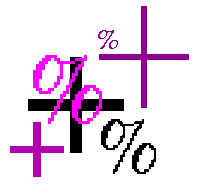


This operator forms a blend of two input images of the same size. Similar to pixel addition, the value of each pixel in the output image is a linear combination of the corresponding pixel values in the input images. The coefficients of the linear combination are user-specified and they define the ratio by which to scale each image before combining them. These proportions are applied such that the output pixel values do not exceed the maximum pixel value.
The resulting image is calculated using the formula
 and
and  are the two input images. In
some applications
  can also be a constant, thus
allowing a constant offset value to be added to a single image.
X is the blending ratio which determines the influence of each input image in the output. X can either be a constant factor for all pixels in the image or can be determined for each pixel separately using a mask. The size of the mask must then be identical with the size of the images.
Some implementations only support graylevel images. If multi-spectral images are supported the calculation is done for each band separately.
The image
shows a simple flat dark object against a light background. Applying the Canny edge detector to this image we obtain
We get
if we apply the blending operator with X =
0.5, where the original image is  and the edge image
is
  . The result clearly shows the disadvantage of
image blending over image addition: since each of the input images is
scaled with 0.5 before they are added up, the contrast of each image
is halved. That is why it is hard to see the difference between the
object and the background of the original image. If the contrast in
one image is more important than the other, we can improve the result
by choosing a blending ratio other than 0.5, thus keeping more of the
contrast in the image where it is needed. To get
the same two images as above were blended with X=0.7.
The bad result in the first example is mainly due to the low initial contrast in the input images. So, we will have a better result if the input images are of high contrast. To produce
the input images were contrast-enhanced with contrast stretching and then blended with X = 0.5. Although this already yields a better result, we still lose some contrast with respect to the original input images.
To maintain the full contrast in the output image we can define a
special mask. The mask is made by thresholding the
edge image at a pixel value of 128 and setting the non-zero values to
one. Now, we blend the graylevel edge image (now corresponding to
 ) and the original image using the thresholded image
as a blending mask X(i,j). The image
shows the result, which is identical to the one achieved with image addition, but now achieved via a slightly simpler process.
Blending can also be used to achieve nice effects in photographs. We obtained
by blending
with the resized version of
using the X=0.5.
You can interactively experiment with this operator by clicking here.
and
using skeletonization. Assess the result by combining the two images using the blending operator.
E. Davies Machine Vision: Theory, Algorithms and Practicalities, Academic Press, 1990, Chap. 2.
Specific information about this operator may be found here.
More general advice about the local HIPR installation is available in the Local Information introductory section.


