The Bio-PEPA Eclipse Plug-inUser Manual: Functional Rates

A.4 Functional Rates

The concrete syntax for the functional rates, as accepted by the plug-in, is as follows [14]:

$\begin{array}{r} \mathsf{kineticLawOf} \; ID : expression’ ; \end{array}$

$\begin{array}{r} ID = [\; expression’ \; ]; \end{array}$

where $expression’$ extends the previous expression statement (see section A.3) to also include pre-defined kinetic rates as shown in [14]:

$\begin{array}{r} expression’ = expression \; | \; \mathsf{fMA}(expr ) \; |\; \mathsf{fMM}(expr, expr) \end{array}$

where $\mathsf{fMA}$ and $\mathsf{fMM}$ stand for mass-action and Michealis-Menten, respectively; additional functions specific to commonly found rates in the biological domain [14]:

Mass-action takes one parameter, r, with the overall rate for the reaction being the product of the rate and the population counts of all the reactants and modifier species involved in the reaction e.g. fMA(r), where the reaction involves species $S_1$ and $S_2$ which interact to form $S_3$ , would equate to a rate of $r * S_1 * S_2$ (assuming stoichiometric coefficients of one). If instead the reaction only involved $S_1$ as a reactant then the corresponding rate would be $r * S_1$ .
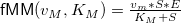
Michaelis-Menten takes two parameters, $v_ M$ and $K_ M$ and requires a set number of species to perform specific roles within the reaction. One species is required to act as a reactant ( $S$ ), another as the enzyme ( $E$ ) and the last as the product ( $P$ ). The ordering of the parameters, along with the associated rate can be seen below.
$\begin{array}{r} \mathsf{fMM}(v_ M, K_ M) = \frac{v_ m*S*E}{K_{M}+S} \end{array}$

Some examples of functional rates definitions are shown here:

`a1`	`=`	`[ r1 * A * B ];`	from `a-b-c.biopepa` model
`kineticLawOf a1`	`:`	`r1 * A * B;`	equivalent definition
`a1`	`=`	`[ fMA(r1) ];`	mass-action kinetics example
`kineticLawOf a1`	`:`	`fMA(r1);`	equivalent definition
`a1`	`=`	`[ v/(KM+P2) ];`	Michaelis-Menten kinetics example
`kineticLawOf a1`	`:`	`v/(KM+P2);`	equivalent definition

In later sections (A.7 - A.10), we will see more examples of both mass-action and Michaelis-Menten kinetics (see section A.8 and section A.10), as well as other functional rates definitions.