Estimating ASSEMBLY Reference Frames

If a set of model vectors (e.g. surface normals) can be paired with corresponding data vectors, then a least-squared error estimate of the transformation could be estimated using methods like that of Faugeras and Hebert [63]. This integrates all evidence uniformly. The method described below estimates reference frame parameters from smaller amounts of evidence, which is then integrated using the parameter space intersection method described above. The justification for this approach was that it is incremental and shows the intermediate results more clearly. It can also integrate evidence hierarchically from previously located subcomponents.

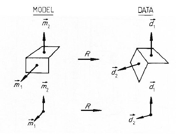
Each data surface has a normal that, given correspondence with a particular model SURFACE, constrains the orientation of the ASSEMBLY to a single rotational degree-of-freedom about the normal. A second, non-parallel, surface normal then fixes the object's rotation. The calculation given here is based on transforming a pair of model SURFACE normals onto a data pair. The model normals have a particular fixed angle between them. Given that the data normals must meet the same constraint, the rotation that transforms the model vectors onto the data vectors can be algebraically determined. Figure 9.6 illustrates the relationships.

Figure 9.6: Rotating Model Normals to Derive the Reference Frame

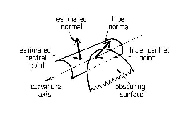
Use of surface normals is reasonable only for nearly planar surfaces. For cylindrical or ellipsoidal surfaces, normals at the central points on the data and model surfaces can be computed and compared, but: (1) small displacements of the measurement point on surfaces with moderate curvature lead to significant changes in orientation, and (2) occlusion makes it impossible to accurately locate corresponding points. Fortunately, highly curved surfaces often have a curvature axis that is more accurately estimated and is not dependent on precise point positions nor is it affected by occlusion. Figure 9.7 illustrates these points.

Figure 9.7: Axis Stability on Cylindrical Surfaces

A third approach uses the vector through the central points in the surfaces, which is most useful when the surfaces are widely separated. Then, variations in point placement (e.g. due to occlusion) will cause less significant effects in this vector's orientation.

Given these techniques, two surface patches give rise to eight orientation estimation cases:

1. Two planes with surface normals not parallel: use the data normals paired to the model normals.
2. Two planes with surface normals nearly parallel: use one data normal paired to the model normal and the second vector from paired central points.
3. Any shape and a generic surface (i.e. with two non-zero curvatures), normals not parallel: use the data normals paired to the model normals.
4. Any shape and a generic surface, normals nearly parallel: use one data normal paired to the model normal and the second vector from paired central points.
5. Plane and cylinder, cylinder axis not parallel to plane normal: use paired plane data and model normals, paired cylinder data and model axes.
6. Plane and cylinder, cylinder axis nearly parallel to plane normal: use the data normals paired to the model normals.
7. Two cylinders, axes not parallel: use data axes paired with model axes.
8. Two cylinders, axes nearly parallel: use one data axis paired to the model axis and the second vector from paired central points.

After feature pairing, the rotation angles are estimated. Unfortunately, noise and point position errors mean that the interior angles between the pairs of vectors are only approximately the same, which makes exact algebraic solution impossible. So, a variation on the rotation method was used. A third pair of vectors, the cross product of each original pair, are calculated and have the property of being at right angles to each of the original pairs:

Let:
	$\vec{d}_1$, $\vec{d}_2$ be the data normals
	$\vec{m}_1$, $\vec{m}_2$ be the model normals
Then, the cross products are:
	$\vec{c_d} = \vec{d}_1 \times \vec{d}_2$
	$\vec{c_m} = \vec{m}_1 \times \vec{m}_2$

From $\vec{d}_1$ and $\vec{c_d}$ paired to $\vec{m}_1$ and $\vec{c_m}$ an angular parameter estimate can be algebraically calculated. Similarly, $\vec{d}_2$ and $\vec{c_d}$ paired to $\vec{m}_2$ and $\vec{c_m}$ gives another estimate, which is then integrated using the parameter space intersection technique.

Fan et al. [61] used a somewhat similar paired vector reference frame estimation technique for larger sets of model-to-data vector pairings, except that they picked the single rotation estimate that minimized an error function, rather than integrated all together. This often selects a correct rotation from a set of pairings that contains a bad pairing, thus allowing object recognition to proceed.

Before the rotation is estimated from a pair of surfaces, a fast compatibility test is performed, which ensures that the angle between the data vectors is similar to that between the model vectors. (This was similar to the angular pruning of Faugeras and Hebert [63]). The test is:

Let:
	$\vec{d}_1$, $\vec{d}_2$ be the data normals
	$\vec{m}_1$, $\vec{m}_2$ be the model normals
If:
	$\mid (\vec{d}_1 \circ \vec{d}_2) - (\vec{m}_1 \circ \vec{m}_2) \mid < \tau_c$	($\tau_c = 0.3$)
Then, the vector pairs are compatible.

The global translation estimates come from individual surfaces and substructures. For surfaces, the estimates come from calculating the translation of the nominal central point of the rotated model SURFACE to the estimated central point of the observed surface. Occlusion affects this calculation by causing the image central point to not correspond to the projected model point, but the errors introduced by this technique were within the level of error caused by mis-estimating the rotational parameters. The implemented algorithm for SURFACEs is:

Let:
	$G$ be the transformation from the ASSEMBLY's coordinate system to that of the camera
	$A$ be the transformation from the SURFACE's coordinate system to that of the ASSEMBLY
Then:
	1. Get the estimated global rotation for that SURFACE: ($GA$)
	2. Rotate the central point ($\vec{p}$) of the model SURFACE: ( $\vec{v}_1 = GA\vec{p}$)
	3. Calculate the three dimensional location ($\vec{v}_2$) of the image region centroid, inverting its image coordinates using the depth value given in the data
	4. Estimate the translation as $\vec{v}_2 - \vec{v}_1$