Common Names: Laplacian, Laplacian of Gaussian, LoG, Marr Filter
The Laplacian is a 2-D isotropic measure of the 2nd
spatial derivative of an image. The Laplacian of an image highlights
regions of rapid intensity change and is therefore often
used for edge detection (see zero crossing edge
detectors). The Laplacian is often applied to an image that has first
been smoothed with something approximating a Gaussian
smoothing filter in order to reduce its sensitivity to noise, and
hence the two variants will be described together here. The operator
normally takes a single graylevel image as input and produces another
graylevel image as output.
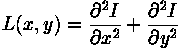
The Laplacian L(x,y) of an image with pixel intensity values I(x,y) is given by:
This can be calculated using a
convolution filter.
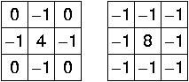
Since the input image is represented as a set of discrete pixels, we have to find a discrete convolution kernel that can approximate the second derivatives in the definition of the Laplacian. Two commonly used small kernels are shown in Figure 1.
Figure 1 Two commonly used discrete approximations to the Laplacian filter. (Note, we have defined the Laplacian using a negative peak because this is more common; however, it is equally valid to use the opposite sign convention.)
Using one of these kernels, the Laplacian can be calculated using standard convolution methods.
Because these kernels are approximating a second derivative measurement on the image, they are very sensitive to noise. To counter this, the image is often Gaussian smoothed before applying the Laplacian filter. This pre-processing step reduces the high frequency noise components prior to the differentiation step.
In fact, since the convolution operation is associative, we can convolve the Gaussian smoothing filter with the Laplacian filter first of all, and then convolve this hybrid filter with the image to achieve the required result. Doing things this way has two advantages:
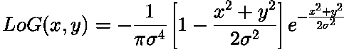
The 2-D LoG function centered on zero and with Gaussian standard
deviation  has the form:
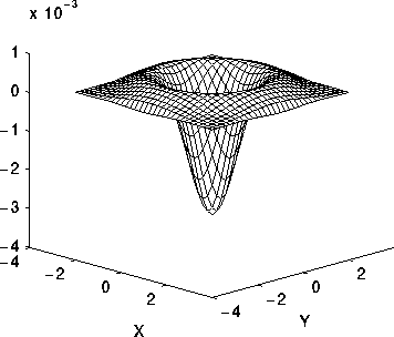
and is shown in Figure 2.
Figure 2 The 2-D Laplacian of Gaussian (LoG) function. The x and y axes are marked in standard deviations (
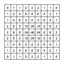
A discrete kernel that approximates this function (for a Gaussian
= 1.4) is shown in Figure 3.
Figure 3 Discrete approximation to LoG function with Gaussian
Note that as the Gaussian is made increasingly narrow, the LoG kernel
becomes the same as the simple Laplacian kernels shown in
Figure 1. This is because smoothing with a very narrow
Gaussian ( < 0.5 pixels) on a discrete grid has no
effect. Hence on a discrete grid, the simple Laplacian can be seen as
a limiting case of the LoG for narrow Gaussians.
The LoG operator calculates the second spatial derivative of an image. This means that in areas where the image has a constant intensity (i.e. where the intensity gradient is zero), the LoG response will be zero. In the vicinity of a change in intensity, however, the LoG response will be positive on the darker side, and negative on the lighter side. This means that at a reasonably sharp edge between two regions of uniform but different intensities, the LoG response will be:
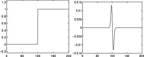
Figure 4 illustrates the response of the LoG to a step edge.
Figure 4 Response of 1-D LoG filter to a step edge. The left hand graph shows a 1-D image, 200 pixels long, containing a step edge. The right hand graph shows the response of a 1-D LoG filter with Gaussian
By itself, the effect of the filter is to highlight edges in an image.
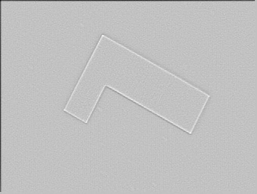
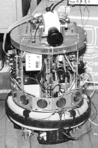
For example,
is a simple image with strong edges.
The image
is the result of applying a LoG filter with
Gaussian = 1.0. A 7×7 kernel was used. Note that
the output contains negative and non-integer values, so for display
purposes the image has been normalized to the range
0 - 255.
If a portion of the filtered, or
gradient, image is added to the original image, then the
result will be to make any edges in the original image much sharper
and give them more contrast. This is commonly used as an enhancement technique
in remote sensing applications.
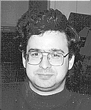
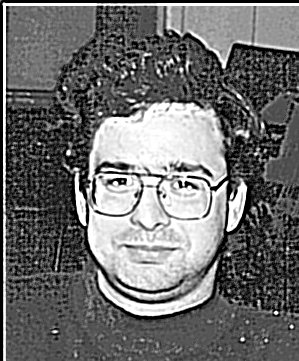
To see this we start with
which is a slightly blurry image of a face.
The image
is the effect of applying an LoG filter with
Gaussian = 1.0, again using a 7×7 kernel.
Finally,
is the result of combining (i.e. subtracting) the filtered image and the original image. Note that the filtered image had to be suitable scaled before combining in order to produce a sensible enhancement. Also, it may be necessary to translate the filtered image by half the width of the convolution kernel in both the x and y directions in order to register the images correctly.
The enhancement has made edges sharper but has also increased the effect of noise. If we simply filter the image with a Laplacian (i.e. use a LoG filter with a very narrow Gaussian) we obtain
Performing edge enhancement using this sharpening image yields the noisy result
(Note that unsharp filtering may produce an equivalent result since it can be defined by adding the negative Laplacian image (or any suitable edge image) onto the original.) Conversely, widening the Gaussian smoothing component of the operator can reduce some of this noise, but, at the same time, the enhancement effect becomes less pronounced.
The fact that the output of the filter passes through zero at edges can be used to detect those edges. See the section on zero crossing edge detection.
Note that since the LoG is an
isotropic filter,
it is not possible to
directly extract edge orientation information from the LoG output in
the same way that it is for other edge detectors such as the
Roberts Cross and Sobel operators.
Convolving with a kernel such as the one shown in Figure 3 can very easily produce output pixel values that are much larger than any of the input pixels values, and which may be negative. Therefore it is important to use an image type (e.g. floating point) that supports negative numbers and a large range in order to avoid overflow or saturation. The kernel can also be scaled down by a constant factor in order to reduce the range of output values.
It is possible to approximate the LoG filter with a filter that is
just the difference of two differently sized Gaussians. Such a filter
is known as a DoG filter (short for
`Difference of Gaussians').
As an aside it has been suggested (Marr 1982) that LoG filters (actually DoG filters) are important in biological visual processing.
An even cruder approximation to the LoG (but much faster to compute)
is the DoB filter (`Difference of Boxes').
This is simply the
difference between two mean filters of different sizes. It
produces a kind of squared-off approximate version of the LoG.
You can interactively experiment with the Laplacian operator by clicking here.
You can interactively experiment with the Laplacian of Gaussian operator by clicking here.
What is the general effect of increasing the Gaussian width? Notice particularly the effect on features of different sizes and thicknesses.
of the underlying Gaussian if
severe truncation is to be avoided.
R. Haralick and L. Shapiro Computer and Robot Vision, Vol. 1, Addison-Wesley Publishing Company, 1992, pp 346 - 351.
B. Horn Robot Vision, MIT Press, 1986, Chap. 8.
D. Marr Vision, Freeman, 1982, Chap. 2, pp 54 - 78.
D. Vernon Machine Vision, Prentice-Hall, 1991, pp 98 - 99, 214.
Specific information about this operator may be found here.
More general advice about the local HIPR installation is available in the Local Information introductory section.
©2003 R. Fisher, S. Perkins,
A. Walker and E. Wolfart.
![]()