Compass Edge Detection
is an alternative approach to the differential gradient edge detection (see the Roberts Cross and Sobel operators). The operation usually outputs two images, one estimating the local edge gradient magnitude and one estimating the edge orientation of the input image.
convolved
with a set of (in general 8) convolution kernels, each of which is sensitive to edges in a different orientation. For each pixel the local edge gradient magnitude is estimated with the maximum response of all 8 kernels at this pixel location:
where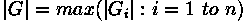
 is the response of the kernel i at the particular pixel position and n is the number of convolution kernels. The local edge orientation is estimated with the orientation of the kernel that yields the maximum response.
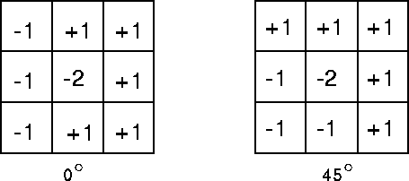
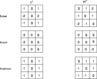
Various kernels can be used for this operation; for the following discussion we will use the Prewitt kernel. Two templates out of the set of 8 are shown in Figure 1:
Figure 1 Prewitt compass edge detecting templates sensitive to edges at 0° and 45°.
The whole set of 8 kernels is produced by taking one of the kernels and rotating its coefficients circularly. Each of the resulting kernels is sensitive to an edge orientation ranging from 0° to 315° in steps of 45°, where 0° corresponds to a vertical edge.
The maximum response |G| for each pixel is the value of the corresponding pixel in the output magnitude image. The values for the output orientation image lie between 1 and 8, depending on which of the 8 kernels produced the maximum response.
This edge detection method is also called edge template matching, because a set of edge templates is matched to the image, each representing an edge in a certain orientation. The edge magnitude and orientation of a pixel is then determined by the template that matches the local area of the pixel the best.
The compass edge detector is an appropriate way to estimate the magnitude and orientation of an edge. Although differential gradient edge detection needs a rather time-consuming calculation to estimate the orientation from the magnitudes in the x- and y-directions, the compass edge detection obtains the orientation directly from the kernel with the maximum response. The compass operator is limited to (here) 8 possible orientations; however experience shows that most direct orientation estimates are not much more accurate.
On the other hand, the compass operator needs (here) 8 convolutions for each pixel, whereas the gradient operator needs only 2, one kernel being sensitive to edges in the vertical direction and one to the horizontal direction.
The result for the edge magnitude image is very similar with both methods, provided the same convolving kernel is used.
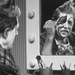
If we apply the Prewitt Compass Operator to
we get two output images. The image
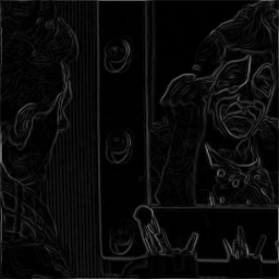
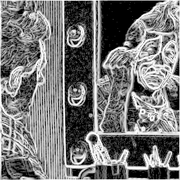
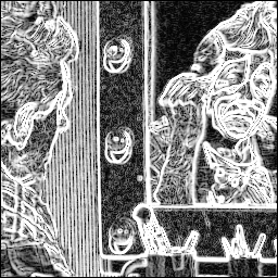
shows the local edge magnitude for each pixel. We can't see much in this image, because the response of the Prewitt kernel is too small. Applying histogram equalization to this image yields
The result is similar to
which was processed with the Sobel differential gradient edge detector and histogram equalized.
The edges in the image can be rather thick, depending on the size of the convolving kernel used. To remove this unwanted effect some further processing (e.g. thinning) might be necessary.
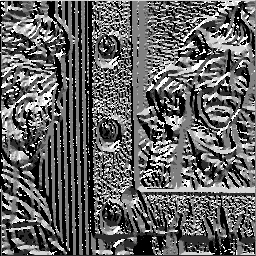
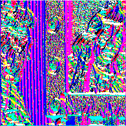
The image
is the graylevel orientation image that was contrast-stretched for a better display. That means that the image contains 8 graylevel values between 0 and 255, each of them corresponding to an edge orientation. The orientation image as a color labeled image (containing 8 colors, each corresponding to one edge orientation) is shown in
The orientation of strong edges is shown very clearly, as for example at the vertical stripes of the wall paper. On a uniform background without a noticeable image gradient, on the other hand, it is ambiguous which of the 8 kernels will yield the maximum response. Therefore a uniform area results in a random distribution of the 8 orientation values.
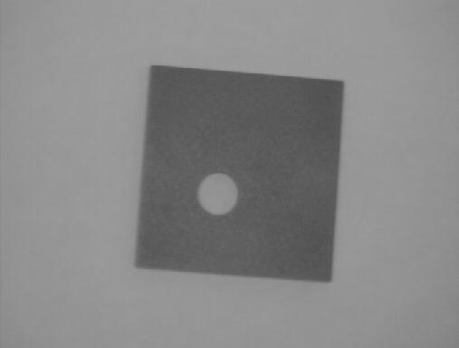
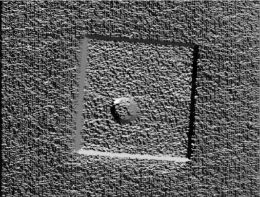
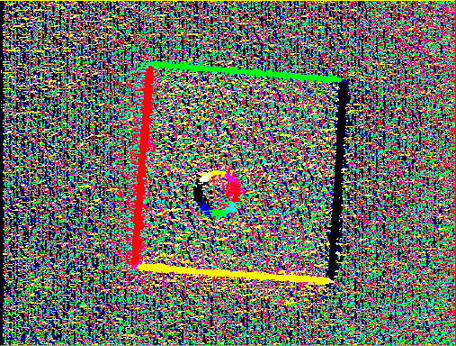
A simple example of the orientation image is obtained if we apply the Compass Operator to
Each straight edge of the square yields a line of constant color (or graylevel). The circular hole in the middle, on the other hand, contains all 8 orientations and is therefore segmented in 8 parts, each of them having a different color. Again, the image is displayed as a normalized graylevel image
and as a colored label image
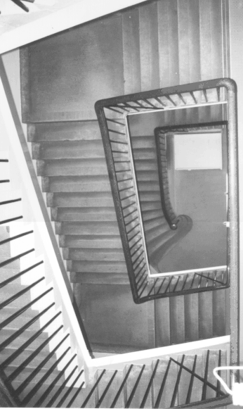
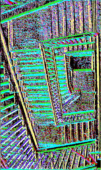
The image
is an image containing many edges with gradually changing orientation. Applying the Prewitt compass operator yields
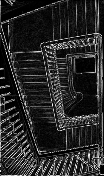
for the edge magnitude and
for the edge orientation. Note that, due to the distortion of the image, all posts along the railing in the lower left corner have a slightly different orientation. However, the operator classifies them in only 3 different classes, since it assigns the same orientation label to edges when the orientation varies within 45°.
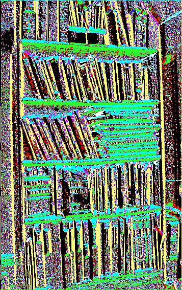
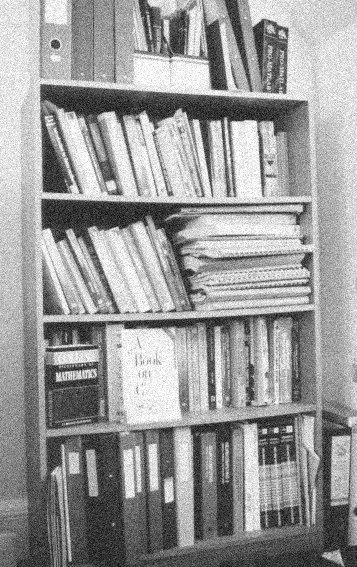
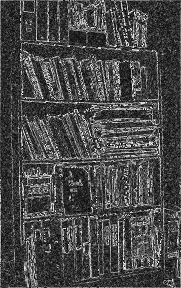
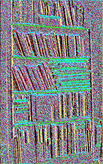
Another image suitable for edge detection is
The corresponding output of the compass edge detector is
and
for the magnitude and orientation, respectively. Like the previous image, this image contains little noise and most of the resulting edges correspond to boundaries of objects. Again, we can see that most of the roughly vertical books were assigned the same orientation label, although the orientation varies by some amount.
We demonstrate the influence of noise on the compass operator by adding Gaussian noise with a standard deviation of 15 to the above image. The image
shows the noisy image. The Prewitt compass edge detector yields
for the edge magnitude and
for the edge orientation. Both images contain a large amount of noise and most areas in the orientation image consist of a random distribution of the 8 possible values.
Figure 2 Some examples for the most common compass edge detecting kernels, each example showing two kernels out of the set of eight.
For every template, the set of all eight kernels is obtained by shifting the coefficients of the kernel circularly.
The result for using different templates is similar; the main difference is the different scale in the magnitude image. The advantage of Sobel and Robinson kernels is that only 4 out of the 8 magnitude values must be calculated. Since each pair of kernels rotated about 180° opposite is symmetric, each of the remaining four values can be generated by inverting the result of the opposite kernel.
You can interactively experiment with this operator by clicking here.
(e.g. by rotating the image about 45° and blending it with the original). Then apply the compass edge operator to the resulting image and examine the edge orientation image. Do the same with an image containing 12 different edge orientations.
E. Davies Machine Vision: Theory, Algorithms and Practicalities, Academic Press, 1990, pp 101 - 110.
R. Gonzalez and R. Woods Digital Image Processing, Addison-Wesley Publishing Company, 1992, p 199.
D. Vernon Machine Vision, Prentice-Hall, 1991, Chap. 5.
Specific information about this operator may be found here.
More general advice about the local HIPR installation is available in the Local Information introductory section.
©2003 R. Fisher, S. Perkins,
A. Walker and E. Wolfart.
![]()